

Post by tympakie on Jul 6, 2020 20:34:20 GMT
Distribution of mining resource abundances on the real Earth.
First of all: this post is not meant as a critique to the game or as a proposal for a change to its dynamics. Rather it would hint at a realistic model, and give some possible reference for economics students playing the game.
It is well known in statistics that “the sizes of things occurring in nature, such as city sizes, heights of mountains, and lengths of rivers” have an asymmetric distribution strongly peaked towards small values and with long tails extending to large values. See the book on Beginning Statistics with Data Analysis by Mosteller, Fienberg and Rourke, 1983, Addison-Wesley, for example.
Let us see some examples for mining resources.
The following histogram plots the data given in Table 2 of a document available from the web pages of the Canadian Government:
www.nrcan.gc.ca/mining-materials/exploration/8294

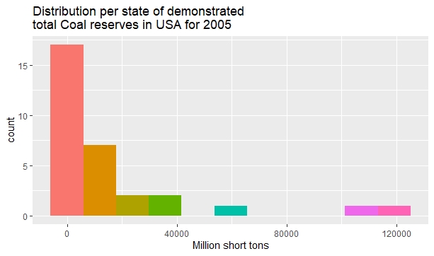
The next histogram plots the distribution of Coal reserves in 31 American States as given in Table D.1 of a book by the American National Research Council:
www.nap.edu/read/11977/chapter/14
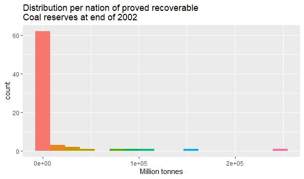
The last histogram is for the total Coal reserves of 73 world nations, as given in Table D.2 of the same book.
Let us remark that all have the same shape.
It is also well known that we can get a more symmetrical distribution by transforming data with logarithms, as the following pictures show for each of the previous sets of data.
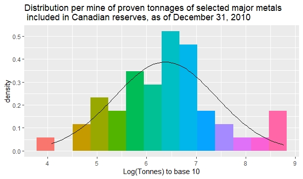
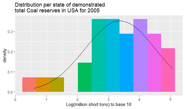
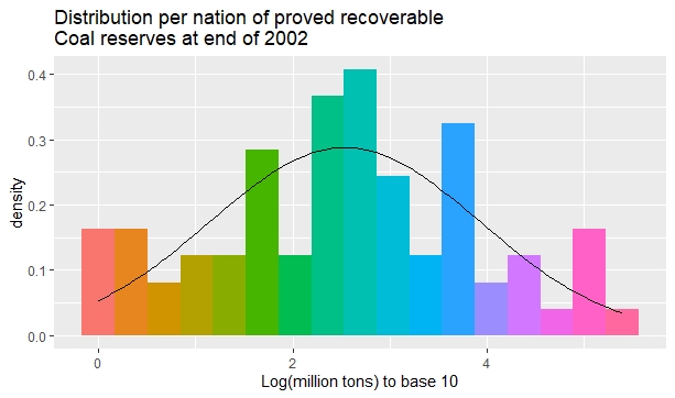
The previous figures also show a superposed Gaussian distribution with the same mean and standard deviation as the colored observed distribution.
For example, for mining resources in Canada, the mean is 6.377035 and the standard deviation is 1.02938.
Is this distribution in the logarithm of abundance a Gaussian one? More or less: The null hypothesis that each sample is taken from an underlying Gaussian distribution cannot be rejected, at a confidence level as low as 90%.
A chi square test for the mining resources in Canada, with 5 bins corresponding to the fifths in an underlying Gaussian population (so that each bin contains about 10 expected data), gives a probability of a larger chi square about 50.3%.
For the Coal resources in 31 American states, a chi square test with 4 bins (so that we have at least one degree of freedom) gives a probability of a larger chi square about 43.4%.
For the Coal resources in 73 world nations, a chi square test with 7 bins gives a probability for a chi square larger than the observed one about 22.1%.
Yearly decrease of reserve abundance in Canadian mineral reserves from 1983 to 2010.
Taken as the life indices (from 2009 to 2010) from the data reported at
www.nrcan.gc.ca/mining-materials/exploration/8294
Nickel: 5.6%
Copper: 4.2%
Zinc: 17%
Lead: 20%
Molybdenum: 3.5%
Silver: 10%
Gold: 11%
First of all: this post is not meant as a critique to the game or as a proposal for a change to its dynamics. Rather it would hint at a realistic model, and give some possible reference for economics students playing the game.
It is well known in statistics that “the sizes of things occurring in nature, such as city sizes, heights of mountains, and lengths of rivers” have an asymmetric distribution strongly peaked towards small values and with long tails extending to large values. See the book on Beginning Statistics with Data Analysis by Mosteller, Fienberg and Rourke, 1983, Addison-Wesley, for example.
Let us see some examples for mining resources.
The following histogram plots the data given in Table 2 of a document available from the web pages of the Canadian Government:
www.nrcan.gc.ca/mining-materials/exploration/8294
The next histogram plots the distribution of Coal reserves in 31 American States as given in Table D.1 of a book by the American National Research Council:
www.nap.edu/read/11977/chapter/14
The last histogram is for the total Coal reserves of 73 world nations, as given in Table D.2 of the same book.
Let us remark that all have the same shape.
It is also well known that we can get a more symmetrical distribution by transforming data with logarithms, as the following pictures show for each of the previous sets of data.
Mining reserves in 48 Canadian mines.
Coal reserves in 31 American states.
Coal reserves in 73 world nations.
The previous figures also show a superposed Gaussian distribution with the same mean and standard deviation as the colored observed distribution.
For example, for mining resources in Canada, the mean is 6.377035 and the standard deviation is 1.02938.
Is this distribution in the logarithm of abundance a Gaussian one? More or less: The null hypothesis that each sample is taken from an underlying Gaussian distribution cannot be rejected, at a confidence level as low as 90%.
A chi square test for the mining resources in Canada, with 5 bins corresponding to the fifths in an underlying Gaussian population (so that each bin contains about 10 expected data), gives a probability of a larger chi square about 50.3%.
For the Coal resources in 31 American states, a chi square test with 4 bins (so that we have at least one degree of freedom) gives a probability of a larger chi square about 43.4%.
For the Coal resources in 73 world nations, a chi square test with 7 bins gives a probability for a chi square larger than the observed one about 22.1%.
Yearly decrease of reserve abundance in Canadian mineral reserves from 1983 to 2010.
Taken as the life indices (from 2009 to 2010) from the data reported at
www.nrcan.gc.ca/mining-materials/exploration/8294
Nickel: 5.6%
Copper: 4.2%
Zinc: 17%
Lead: 20%
Molybdenum: 3.5%
Silver: 10%
Gold: 11%